FindStadiums

Fine-tuning OlmoEarth and Other Models to Find Stadiums

This example walks through fine-tuning OlmoEarth and other models to find stadiums.

Compared to other examples like FinetuneOlmoEarth, there are two unique aspects to this example:

• We will fine-tune with multiple remote sensing foundation models, and compare their performance.
• We will start with source data consisting of the locations of 253 stadiums in the US, and show how to use it to train a segmentation model. There are two key challenges associated with this data: (1) instead of dense segmentation masks, we only have sparse point labels; and (2) we only have positive labels.

Training Data

We will start with a CSV of stadiums in docs/examples/FindStadiums/stadiums.csv, which is originally from gboeing/data-visualization.

It consists of stadium points like this:

stadium	city	state	team	conference	capacity	built	expanded	div	latitude	longitude
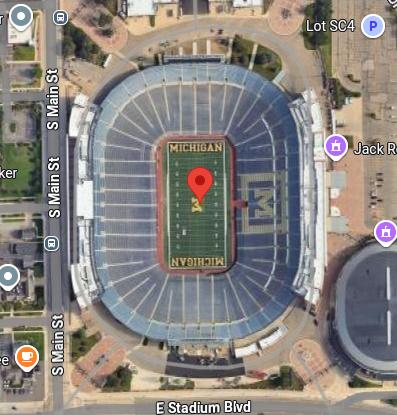
Michigan Stadium	Ann Arbor	MI	Michigan	Big Ten	107601	1927	2015	fbs	42.2659	-83.7487
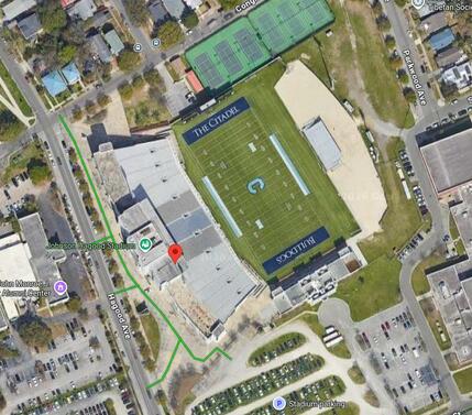
Johnson Hagood Stadium	Charleston	South Carolina	The Citadel Bulldogs	Southern	21000	1948	2008	fcs	32.7933	-79.9564
Beaver Stadium	University Park	PA	Penn State	Big Ten	106572	1960	2001	fbs	40.8122	-77.8562

One issue with the data is that, while some of these coordinates are at the center of the stadium, others are off to the side:

Data Strategy

We want to train a model to classify each pixel as "stadium" or "background". As mentioned above, there are two key challenges with the data:

1. Instead of dense segmentation masks, we only have sparse point labels.
2. We only have positive labels.

A typical approach for addressing the first challenge is to mask the loss everywhere except at the pixel corresponding to the label, and input random crops where the label appears at a random position within the crop. This way, the segmentation model is trained to output a reasonable prediction at each output pixel. We could also train a classification model, but this does not scale well if we want to perform inference to compute per-pixel predictions over large areas (needs one forward pass per pixel).

To achieve this with 64x64 input crops in rslearn, we would create a 128x128 window centered at the labeled point, and programmatically add a 128x128 label GeoTIFF where all pixels are NODATA except the pixel in the center. Then, in the model configuration, we can set crop_size: 64; this way, the random cropping will choose crops that have the labeled point at random pixel positions.

To also address the second challenge, we adapt this approach. Specifically, we will use the area around the stadium as negatives, and just assume that there are no other stadiums in its vicinity.

To handle stadiums spanning many pixels and the coordinates not being exact, we will make two more modifications:

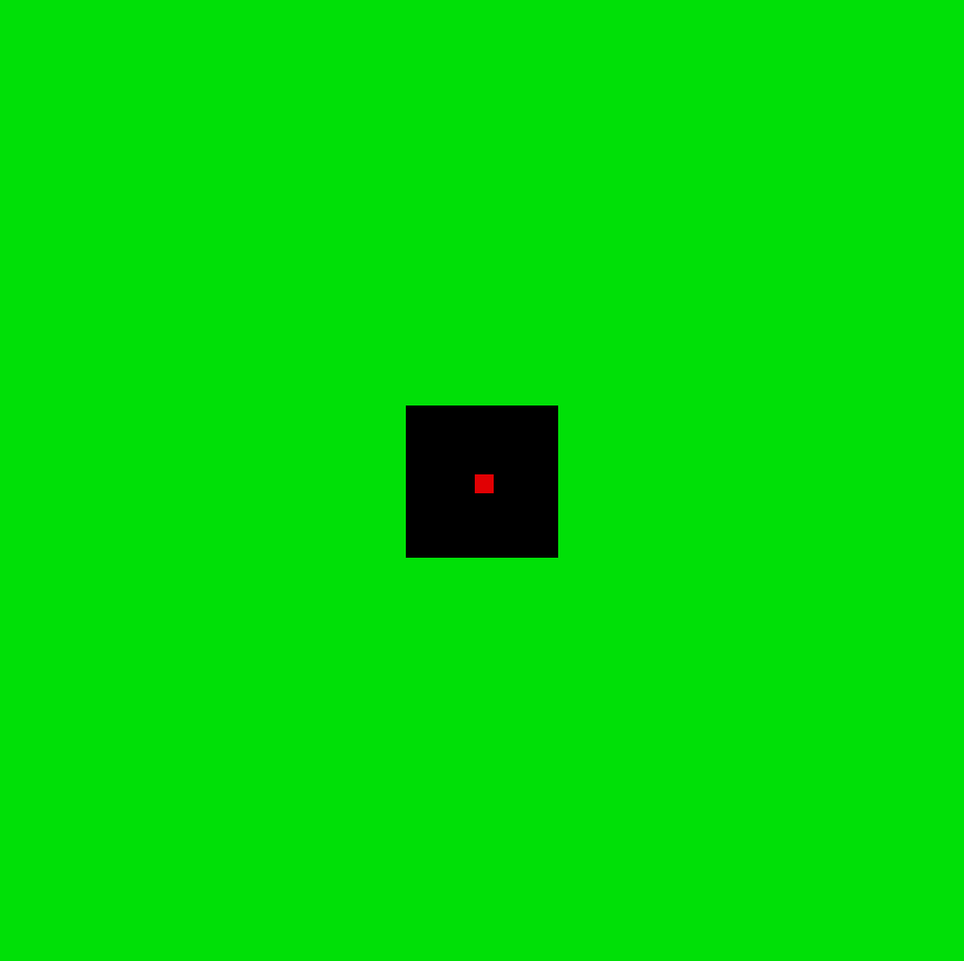
• Instead of just marking the labeled pixel as "stadium", we mark the 5x5 neighborhood around the point.
• Then, around that, we put a 40x40 NODATA buffer. This masks out the loss for pixels close to the stadium that we are not sure about due to the coordinate imprecision.
• Finally, we assume the rest of the area is "background".

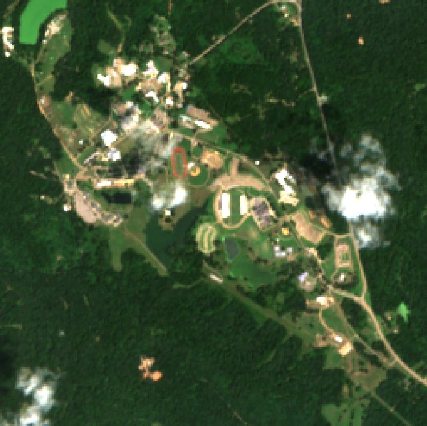
Here is an example label and corresponding Sentinel-2 image. Red is "stadium", green is "background", and black is nodata (will have masked loss).

Create Windows

Create a new directory to contain the rslearn dataset:

mkdir ./dataset
export DATASET_PATH=./dataset

Write the dataset config below to ./dataset/config.json. Besides specifying layers for the labels and prediction outputs, it also includes a Sentinel-2 layer that rslearn should populate with up to three Sentinel-2 images per window, with one per thirty-day period of each window's time range.

{
  "layers": {
    "label": {
      "band_sets": [
        {
          "bands": ["label"],
          "dtype": "uint8",
          "nodata_value": 0
        }
      ],
      "type": "raster"
    },
    "output": {
      "band_sets": [
        {
          "bands": ["prob"],
          "dtype": "float32"
        }
      ],
      "type": "raster"
    },
    "sentinel2": {
      "band_sets": [
        {
          "bands": ["B01", "B02", "B03", "B04", "B05", "B06", "B07", "B08", "B8A", "B09", "B11", "B12"],
          "dtype": "uint16"
        }
      ],
      "data_source": {
        "class_path": "rslearn.data_sources.planetary_computer.Sentinel2",
        "ingest": false,
        "init_args": {
          "harmonize": true,
          "query": {"eo:cloud_cover": {"lt": 50}},
          "sort_by": "eo:cloud_cover"
        },
        "query_config": {
          "max_matches": 3,
          "per_period_mosaic_reverse_time_order": false,
          "period_duration": "30d"
        }
      },
      "type": "raster"
    }
  }
}

The script below implements the data strategy discussed above. We skip all three rows in Washington state since we will test the model on a portion of Seattle, WA later. The CSV uses both WA and Washington in its state column, so the script handles both spellings while retaining Washington, D.C. The 250 resulting windows all share the same 90-day time range, from 1 June 2025 to 30 August 2025.

import csv
import hashlib
import os
import re
from datetime import UTC, datetime

import numpy as np
import shapely
import tqdm
from upath import UPath

from rslearn.const import WGS84_PROJECTION
from rslearn.dataset import Dataset, Window
from rslearn.utils.geometry import STGeometry
from rslearn.utils.get_utm_ups_crs import get_utm_ups_projection
from rslearn.utils.raster_array import RasterArray
from rslearn.utils.raster_format import GeotiffRasterFormat

CSV_PATH = "docs/examples/FindStadiums/stadiums.csv"
WINDOW_SIZE = 256
RESOLUTION = 10
TIME_RANGE = (
  datetime(2025, 6, 1, tzinfo=UTC),
  datetime(2025, 8, 30, tzinfo=UTC),
)
VAL_RATIO = 0.2

# We assign nearby points to the same split based on a coarse geographic region.
def location_to_split(lon: float, lat: float) -> str:
  region = f"{int(lon // 2)}_{int(lat // 2)}"
  h = int(hashlib.sha256(region.encode()).hexdigest(), 16)
  return "val" if (h % 100) < VAL_RATIO * 100 else "train"

# Stadium names are not unique, so include the team in each window name.
def get_window_name(row: dict[str, str]) -> str:
  value = f"{row['stadium']}_{row['team']}"
  return re.sub(r"[^A-Za-z0-9]+", "_", value).strip("_")

# Read the points in the CSV.
# The columns include "state", "longitude", "latitude", and "stadium".
with open(CSV_PATH) as f:
  rows = [
    row
    for row in csv.DictReader(f)
    if row["state"].strip() not in {"WA", "Washington"}
  ]

# Initialize a Dataset object that represents the entire rslearn dataset.
dataset = Dataset(UPath(os.environ["DATASET_PATH"]))

split_counts: dict[str, int] = {}
for row in tqdm.tqdm(rows):
  # For each row in the CSV, start by extracting the columns we want.
  lon = float(row["longitude"])
  lat = float(row["latitude"])
  window_name = get_window_name(row)

  # Assign nearby stadiums to the same train or val split.
  split = location_to_split(lon, lat)
  split_counts[split] = split_counts.get(split, 0) + 1

  # OlmoEarth expects inputs to be at 10 m/pixel in UTM projection. We first
  # find the appropriate UTM projection for this location. In addition to the
  # CRS, the Projection also specifies the m/pixel resolution, which is
  # RESOLUTION=10 here.
  projection = get_utm_ups_projection(lon, lat, RESOLUTION, -RESOLUTION)

  # Now convert the lon/lat to pixel coordinates in that projection. (Pixel
  # coordinates are just CRS coordinates divided by the resolution.) The
  # STGeometry specifies the Projection (CRS + resolution), a shapely geometry
  # in pixel coordinates, and an optional time range (omitted here).
  src_geom = STGeometry(WGS84_PROJECTION, shapely.Point(lon, lat), None)
  # STGeometry.to_projection re-projects the geometry to another projection by
  # transforming each vertex. dst_geom.shp is in pixel coordinates in the
  # target projection.
  dst_geom = src_geom.to_projection(projection)
  cx, cy = int(dst_geom.shp.x), int(dst_geom.shp.y)

  # Compute bounds so that the stadium will be at the center.
  bounds = (cx - WINDOW_SIZE // 2, cy - WINDOW_SIZE // 2, cx + WINDOW_SIZE // 2, cy + WINDOW_SIZE // 2)

  # Create the window. The Window object represents one rslearn window
  # (spatiotemporal bounding box). When we call Window.save, it creates a new
  # folder corresponding to the window in
  # {DATASET_PATH}/windows/{group_name}/{window_name}, and writes the
  # projection, bounds, time range, and other details to metadata.json in that
  # folder.
  window = Window(
    storage=dataset.storage,
    group="default",
    name=window_name,
    projection=projection,
    bounds=bounds,
    time_range=TIME_RANGE,
    options={"split": split},
    data_factory=dataset.window_data_storage_factory,
  )
  window.save()

  # Most of the label is "background" (2).
  label = np.full((1, WINDOW_SIZE, WINDOW_SIZE), 2, dtype=np.uint8)
  mid = WINDOW_SIZE // 2
  # Create a 40x40 NODATA (0) buffer in the center.
  label[:, mid - 20 : mid + 20, mid - 20 : mid + 20] = 0
  # And set the middle 5x5 to "stadium" (1).
  label[:, mid - 2 : mid + 3, mid - 2 : mid + 3] = 1

  # Finally, write the label raster through the window's configured data
  # storage. The projection and bounds must describe the array being written.
  with window.data.open_layer_writer("label") as writer:
    writer.write_raster(
      ["label"],
      GeotiffRasterFormat(),
      projection,
      bounds,
      RasterArray(chw_array=label),
    )
  window.mark_layer_completed("label")

print(f"Done: {split_counts}")

This creates a 256x256 window at 10 m/pixel centered at each stadium point. Then, the script writes a label raster corresponding to each window.

Materialize the Dataset

Materialize the dataset to download aligned Sentinel-2 images. The label layer is already complete because the script wrote it directly; these commands populate the layers that have a data source defined.

rslearn dataset prepare --root $DATASET_PATH
rslearn dataset materialize --root $DATASET_PATH

Visualize one of the GeoTIFFs:

qgis $DATASET_PATH/windows/default/Eddie_Robinson_Stadium_Grambling_State_Tigers/layers/sentinel2/B01_B02_B03_B04_B05_B06_B07_B08_B8A_B09_B11_B12/geotiff.tif $DATASET_PATH/windows/default/Eddie_Robinson_Stadium_Grambling_State_Tigers/layers/label/label/geotiff.tif

Train with OlmoEarth-v1-Tiny

Now we can train a model on the Sentinel-2 images and labels.

Create a file model.yaml with the model config below. We configure the model to apply OlmoEarth-v1-Tiny on 64x64 random crops from the 256x256 windows. Note that many crops will see all negative pixels, but some will intersect with the stadium points in the centers of windows.

model:
  class_path: rslearn.train.lightning_module.RslearnLightningModule
  init_args:
    model:
      class_path: rslearn.models.singletask.SingleTaskModel
      init_args:
        encoder:
          - class_path: rslearn.models.olmoearth_pretrain.model.OlmoEarth
            init_args:
              model_id: OLMOEARTH_V1_TINY
              patch_size: 4
        decoder:
          # The encoder produces a feature map at 1/4 the input resolution. We
          # use UNetDecoder to upsample back to the input resolution. It doesn't
          # apply a true UNet here since we only have one feature resolution,
          # but it still does the upsampling that we need.
          - class_path: rslearn.models.unet.UNetDecoder
            init_args:
              in_channels: [[4, 192]]
              out_channels: 3
              num_channels: {4: 192, 2: 128, 1: 64}
          - class_path: rslearn.train.tasks.segmentation.SegmentationHead
            init_args:
              # Use 10x weight for stadium class since most pixels are
              # background.
              weights: [1, 10, 1]
    optimizer:
      class_path: rslearn.models.olmoearth_pretrain.optimizer.LayerDecayAdamW
      init_args:
        lr: 0.0001
    scheduler:
      class_path: rslearn.train.scheduler.PlateauScheduler
      init_args:
        factor: 0.2
        patience: 2
        min_lr: 0
        cooldown: 10
data:
  class_path: rslearn.train.data_module.RslearnDataModule
  init_args:
    path: ${DATASET_PATH}
    inputs:
      sentinel2_l2a:
        data_type: raster
        layers: ["sentinel2", "sentinel2.1", "sentinel2.2"]
        bands: ["B01", "B02", "B03", "B04", "B05", "B06", "B07", "B08", "B8A", "B09", "B11", "B12"]
        passthrough: true
        dtype: FLOAT32
        load_all_layers: true
      targets:
        data_type: raster
        layers: ["label"]
        bands: ["label"]
        is_target: true
        dtype: INT32
    task:
      class_path: rslearn.train.tasks.segmentation.SegmentationTask
      init_args:
        # We use three classes but reserve the first for NODATA. By setting
        # nodata_value, we ensure the loss is masked at those pixels.
        num_classes: 3
        nodata_value: 0
        # When we apply the model, we will show output probabilities for the
        # stadium class (class 1).
        output_probs: true
        output_class_idx: 1
        metric_kwargs:
          average: micro
    batch_size: 4
    num_workers: 4
    use_in_memory_dataset: true
    default_config:
      groups: ["default"]
      transforms:
        - class_path: rslearn.models.olmoearth_pretrain.norm.OlmoEarthNormalize
          init_args:
            band_names:
              sentinel2_l2a: ["B01", "B02", "B03", "B04", "B05", "B06", "B07", "B08", "B8A", "B09", "B11", "B12"]
    train_config:
      crop_size: 64
      tags:
        split: train
      transforms:
        - class_path: rslearn.models.olmoearth_pretrain.norm.OlmoEarthNormalize
          init_args:
            band_names:
              sentinel2_l2a: ["B01", "B02", "B03", "B04", "B05", "B06", "B07", "B08", "B8A", "B09", "B11", "B12"]
        - class_path: rslearn.train.transforms.flip.Flip
          init_args:
            image_selectors: ["sentinel2_l2a", "target/classes", "target/valid"]
    val_config:
      crop_size: 64
      load_all_crops: true
      tags:
        split: val
    test_config:
      crop_size: 64
      load_all_crops: true
      tags:
        split: val
    predict_config:
      crop_size: 64
      overlap_pixels: 16
      load_all_crops: true
      groups: ["predict"]
      skip_targets: true
      transforms:
        - class_path: rslearn.models.olmoearth_pretrain.norm.OlmoEarthNormalize
          init_args:
            band_names:
              sentinel2_l2a: ["B01", "B02", "B03", "B04", "B05", "B06", "B07", "B08", "B8A", "B09", "B11", "B12"]
trainer:
  max_epochs: 20
  callbacks:
    - class_path: lightning.pytorch.callbacks.LearningRateMonitor
      init_args:
        logging_interval: epoch
    - class_path: rslearn.train.prediction_writer.RslearnWriter
      init_args:
        output_layer: output
        merger:
          class_path: rslearn.train.prediction_writer.RasterMerger
          init_args:
            overlap_pixels: 16
    - class_path: rslearn.train.callbacks.checkpointing.ManagedBestLastCheckpoint
      init_args:
        monitor: val_accuracy
        mode: max

Train the model:

export MANAGEMENT_DIR=./project_data
rslearn model fit \
  --config model.yaml \
  --project_name find_stadiums \
  --run_name olmoearth_tiny \
  --management_dir $MANAGEMENT_DIR

Get Predictions

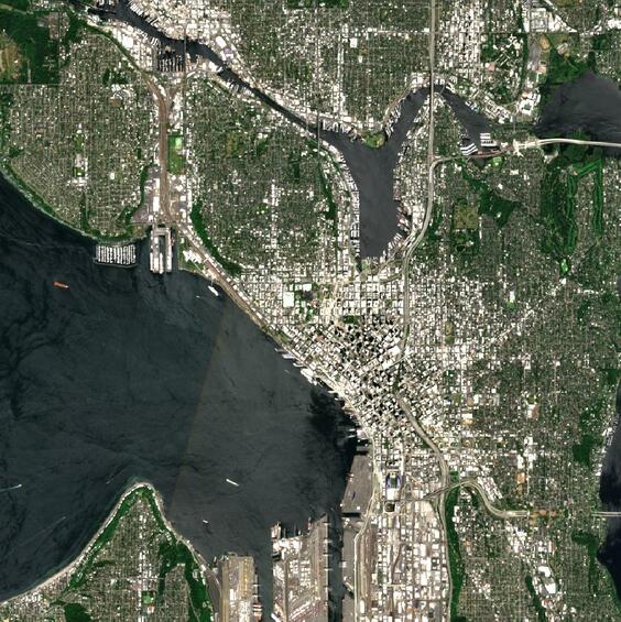
We now apply the model in downtown Seattle. We start by creating a 1024x1024 window for prediction centered at the Space Needle. At 10 m/pixel this covers ~10 km x 10 km, which includes Lumen Field to the south:

rslearn dataset add_windows \
  --root $DATASET_PATH \
  --group predict \
  --utm \
  --resolution 10 \
  --src_crs EPSG:4326 \
  --box=-122.3493,47.6205,-122.3493,47.6205 \
  --window_size 1024 \
  --start 2025-06-01T00:00:00+00:00 \
  --end 2025-08-30T00:00:00+00:00 \
  --name seattle

Prepare and materialize the prediction window:

rslearn dataset prepare --root $DATASET_PATH --group predict
rslearn dataset materialize --root $DATASET_PATH --group predict

Run prediction using the latest checkpoint from training. (We use last.ckpt instead of best.ckpt because, at least in our run, the validation accuracy was highest initially due to the class imbalance. However, the model may still be improving with more training.)

rslearn model predict \
  --config model.yaml \
  --ckpt_path $MANAGEMENT_DIR/find_stadiums/olmoearth_tiny/last.ckpt

Visualize the Sentinel-2 image and model output in QGIS:

qgis $DATASET_PATH/windows/predict/seattle/layers/sentinel2/*/geotiff.tif $DATASET_PATH/windows/predict/seattle/layers/output/*/geotiff.tif

The model picks up on Lumen Field, Husky Stadium, and several smaller sports fields.

Compare Other Remote Sensing Foundation Models

We now compare two other remote sensing foundation models: Clay and Prithvi.

First create these override model config files. We will use these to override the model configured in model.yaml with other options.

Create clay.yaml as follows:

model:
  init_args:
    model:
      init_args:
        encoder:
          - class_path: rslearn.models.simple_time_series.SimpleTimeSeries
            init_args:
              encoder:
                class_path: rslearn.models.clay.clay.Clay
                init_args:
                  model_size: LARGE
                  modality: sentinel-2-l2a
              image_keys:
                - sentinel-2-l2a
              num_timesteps_per_forward_pass: 1
        decoder:
          - class_path: rslearn.models.unet.UNetDecoder
            init_args:
              in_channels: [[8, 1024]]
              out_channels: 3
              conv_layers_per_resolution: 1
              num_channels: {8: 1024, 4: 512, 2: 256, 1: 128}
          - class_path: rslearn.train.tasks.segmentation.SegmentationHead
            init_args:
              weights: [1, 10, 1]
    optimizer:
      class_path: rslearn.train.optimizer.AdamW
      init_args:
        lr: 0.0001
data:
  init_args:
    inputs:
      sentinel-2-l2a:
        data_type: raster
        layers: ["sentinel2", "sentinel2.1", "sentinel2.2"]
        bands: ["B02", "B03", "B04", "B05", "B06", "B07", "B08", "B8A", "B11", "B12"]
        passthrough: true
        dtype: FLOAT32
        load_all_layers: true
      targets:
        data_type: raster
        layers: ["label"]
        bands: ["label"]
        is_target: true
        dtype: INT32
    default_config:
      transforms:
        - class_path: rslearn.models.clay.clay.ClayNormalize
    train_config:
      transforms:
        - class_path: rslearn.models.clay.clay.ClayNormalize
        - class_path: rslearn.train.transforms.flip.Flip
          init_args:
            image_selectors: ["sentinel-2-l2a", "target/classes", "target/valid"]
    predict_config:
      transforms:
        - class_path: rslearn.models.clay.clay.ClayNormalize

And create prithvi.yaml as follows:

model:
  init_args:
    model:
      init_args:
        encoder:
          - class_path: rslearn.models.prithvi.PrithviV2
            init_args:
              size: VIT_300
              num_frames: 3
        decoder:
          - class_path: rslearn.models.unet.UNetDecoder
            init_args:
              in_channels: [[1, 1024]]
              out_channels: 3
              conv_layers_per_resolution: 2
              original_size_to_interpolate: [64, 64]
          - class_path: rslearn.train.tasks.segmentation.SegmentationHead
            init_args:
              weights: [1, 10, 1]
    optimizer:
      class_path: rslearn.train.optimizer.AdamW
      init_args:
        lr: 0.0001
data:
  init_args:
    inputs:
      image:
        data_type: raster
        layers: ["sentinel2", "sentinel2.1", "sentinel2.2"]
        bands: ["B02", "B03", "B04", "B8A", "B11", "B12"]
        passthrough: true
        dtype: FLOAT32
        load_all_layers: true
      targets:
        data_type: raster
        layers: ["label"]
        bands: ["label"]
        is_target: true
        dtype: INT32
    default_config:
      transforms:
        - class_path: rslearn.models.prithvi.PrithviNormalize
    train_config:
      transforms:
        - class_path: rslearn.models.prithvi.PrithviNormalize
        - class_path: rslearn.train.transforms.flip.Flip
          init_args:
            image_selectors: ["image", "target/classes", "target/valid"]
    predict_config:
      transforms:
        - class_path: rslearn.models.prithvi.PrithviNormalize

Now train Clay and Prithvi using the override configs:

rslearn model fit \
  --config model.yaml --config clay.yaml \
  --project_name find_stadiums \
  --run_name clay \
  --management_dir $MANAGEMENT_DIR
rslearn model fit \
  --config model.yaml --config prithvi.yaml \
  --project_name find_stadiums \
  --run_name prithvi \
  --management_dir $MANAGEMENT_DIR

Run predictions with each model:

cp $DATASET_PATH/windows/predict/seattle/layers/output/*/geotiff.tif olmoearth.tif
rslearn model predict \
  --config model.yaml --config clay.yaml \
  --ckpt_path $MANAGEMENT_DIR/find_stadiums/clay/last.ckpt
cp $DATASET_PATH/windows/predict/seattle/layers/output/*/geotiff.tif clay.tif
rslearn model predict \
  --config model.yaml --config prithvi.yaml \
  --ckpt_path $MANAGEMENT_DIR/find_stadiums/prithvi/last.ckpt
cp $DATASET_PATH/windows/predict/seattle/layers/output/*/geotiff.tif prithvi.tif

Compare the outputs in QGIS:

qgis $DATASET_PATH/windows/predict/seattle/layers/sentinel2/*/geotiff.tif olmoearth.tif clay.tif prithvi.tif